3.2.2 Calculating the l.u.b of the processor utilization for the Deferrable Server
Theorem
3.3: For a set of m fixed priority tasks ![]() with
with ![]() where
where ![]() is the deferrable server, the least upper bound of the utilization
function is
is the deferrable server, the least upper bound of the utilization
function is 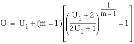 .
Proof
.
Proof
3.2.3 Special Case
This case presumes that all the tasks have approximately
equal periods with a variation within ![]() . As we shall demonstrate,
this arrangement results in a very low least upper bound of the utilization
factor. For such a set of tasks, their repetition periods observe the
following relation.
. As we shall demonstrate,
this arrangement results in a very low least upper bound of the utilization
factor. For such a set of tasks, their repetition periods observe the
following relation. ![]()
In this case, all the periodic tasks must execute within
![]() and
and ![]() as depicted in Figure 3.6 below.
as depicted in Figure 3.6 below.
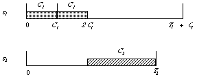
Figure 3.6: Worst case task arrangement.
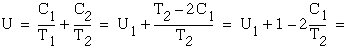
Let's assume the case of two tasks and remember that we are seeking the absolutely worst scenario.
The utilization factor for this case is calculated as follows:
![]() then,
then,

Assuming ![]() (this guarantees that there would always exist time for C2 to execute,
as we shall see subsequently) and since
(this guarantees that there would always exist time for C2 to execute,
as we shall see subsequently) and since ![]() the absolutely possibly worst case, is when
the absolutely possibly worst case, is when ![]() or
or ![]() . Then the lower bound of the utilization is given as
. Then the lower bound of the utilization is given as ![]() .
.
In case that ![]() , then the absolutely worst situation is when
, then the absolutely worst situation is when ![]() does not have enough time
to execute. This can be seen as follows: Suppose that
does not have enough time
to execute. This can be seen as follows: Suppose that ![]() , then
, then 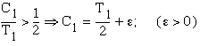 .
.
One can always find T2 such that![]() .
.
This period is within the postulated assumptions i.e.
T2 > T1 (since ![]() > 0) and
> 0) and ![]()
But for any such period, ![]() ; thus
; thus ![]() does not have enough time to run.
does not have enough time to run.
The utilization factor then is given as ![]()
Plotting the utilization factor U in terms of ![]() , one gets
, one gets
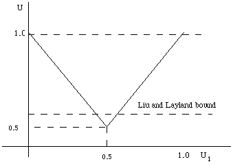
Figure 3.7: The least upper bound of the utilization factor of the deferrable server where the periods of all the tasks are approximately equal.
The analysis outlined above for two tasks can be generalized
for m tasks as follows: If ![]() , then tasks
, then tasks ![]() must execute within
must execute within ![]() and
and ![]() .
.
Thus 
Consider now a new aggregate task ![]() with
with  and
and ![]() .
.
Since ![]() then
then
Thus 
Therefore, for any set of m tasks, we can always construct
a set of two tasks which has a utilization factor ![]() that is always less than the utilization factor U of the set of m tasks.
Thus, the least upper bound of the utilization factor for the m tasks
is exactly that of the case of two tasks as discussed earlier.
that is always less than the utilization factor U of the set of m tasks.
Thus, the least upper bound of the utilization factor for the m tasks
is exactly that of the case of two tasks as discussed earlier.
3.2.4 Experimental Results
The two policies together with standard polling and aperiodic-tasks-in-the-background were simulated to study the sensitivity of the response times to the length of the period of the periodic server.
The aperiodic tasks were assumed to be Poisson distributed
with constant mean inter-arrival time (![]() ) and mean run time (r). The server task and periodic task environments
were chosen so that the periodic load component was 0.45 and the utilization
of the periodic server was computed from equations (3.5) (Priority Exchange)
and (3.14) (Deferrable Server).
) and mean run time (r). The server task and periodic task environments
were chosen so that the periodic load component was 0.45 and the utilization
of the periodic server was computed from equations (3.5) (Priority Exchange)
and (3.14) (Deferrable Server).
Denoting by PLPE and PLDS the processor utilization due to the periodic tasks for the Priority Exchange and Deferrable Server cases respectively, we have from (3.5) and (3.14).
![]() and
and  . Then
![]() and
and 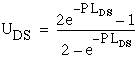 .
.
Setting ![]() , then
, then ![]() and
and ![]() .
.
The simulations used ![]() and
and ![]() for the utilization factors of the periodic servers. The results appear
in Figure 3.8.
for the utilization factors of the periodic servers. The results appear
in Figure 3.8.
The response time for the polling server increases as the period of the server increases, and this is expected since the interval between server invocations increases, and thus arriving aperiodic tasks have to wait longer on the average before they are serviced.
For the Priority Exchange and Deferrable Servers, the response time decreases as the period of the server increases, indicating their ability to respond as soon as aperiodic tasks arrive. Observe though that as the period of the server increases, its priority decreases (according to the rate monotonic assignment that governs the periodic environment). Thus, for large periods which correspond to the lowest priority, the response time becomes identical to that of the aperiodic-tasks-in-the-background discipline.
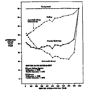
Figure 3.8: The sensitivity of the response time of the aperiodic tasks on the length of the period of the periodic server. (from [5]).